


What would you do if putting a user in the treatment group cost you twice what it costs to put one in control?
I can’t blame you if the first answer that comes to mind is to allocate to the treatment only half the traffic of the control arm. Twice the price per user, so buy half as many; the spend on each arm comes out even. It may feel fair, but it’s not the cheapest answer to that question.
Cost-optimal allocation has to weigh two things at once: how much precision one more subject buys you, and what that subject costs; in a setup where the answer to the second depends on which arm they land in.
“So what?”, you may be thinking. Done properly it can save you anywhere between 5% to 15% of the budget; in other words, from thousands to millions of savings. But at the cost of what? Grab some coffee, and let’s find out when this stops being a free lunch.
In this post, I walk you through:
-
The relevance, given today’s LLM-eager industry, where differing costs across arms are the norm, thinking cost-optimal splits pays off. Discounts, vouchers, cashbacks are other relevant treatments where this show good value.
-
The intuition of cost of the arms plays tug-of-war with the sample variances, and how that leads to twice-the-cost-half-the-traffic NOT being a good answer to the question.
-
The edge cases; for when reality does not fit the math. Experiments don’t run in isolated academic minds. Incentives in business challenge this idea, rightfully.
When the treatment costs money
Personally, I’ve rarely encountered the question of cost-optimal traffic allocation. And I kept thinking: why not? I know the math is not lying, but I also know that experimentation is rarely about the stats alone; like many things organisations, but in particular experimentation, there is a strong business and socio-technical aspect that shapes how it’s done.
Discounting costs money; so do LLMs
In pretty much every industry, recruiting subjects for an experiment is a line in the budget. And sometimes every treatment is the line. In healthcare a new medicine that costs more than the placebo; in economics, in incentive-driven or pay-for-performance designs, every treated subject gets some form of value to nudge them toward the behaviour under study.
In tech, however, there’s a comfortable notion that participants are “free”. There is no one to recruit, convince, or pay; they’re already using your product, so they comply and participate whether they know it or not.
But today half the industry is racing to duct-tape agentic features onto existing products. That’s an open invitation to expensive treatment groups: the AI experience against the old one, where the mere act of treating a user fires off a paid API call. More traditional examples are simply: vouchers, discounts, cash-backs promos, and the like. When a cost differential exists across arms, experimentation programs should start caring.
So, the notion that experimentation is (marginally) free for tech companies, is not too much off, but there is certainly a group of treatments that make cost-optimal designs an interesting path to explore.
What’s the main blocker then? Experimenting with discounts has been around forever. But so has been the need for speed.
Velocity, defaults, and conventions
Velocity is almost everything in digital innovation. Experiments need to come in fast to stay ahead of the competition. We can see that back in two things: the amount of research done in variance reduction techniques, and
If you would be asked: why do we (ideally) split traffic 50/50? The answer would be somewhere along the lines of: that’s when power is highest; ergo, we can find the effect with the shortest runtime possible. That question gets asked far more often than what’s the cost-optimal split?
The pull towards runtime/sensitivity is already baked into traditions. Without a clear protocol, or understanding, on how to govern the traffic split, it’s easy to default to standard reasoning like the 50/50. It has helped in most cases.
It happens to be that a cost-optimal is not per se the one that leads to highest precision, and lowest runtimes. So optimising one objective, means undermining the other one. It’s tug-of-war between cost and velocity. Deciding which one to optimise requires clear understanding of the constraints and priorities; budget, experiment goal, committed timelines, etc. It’s not just a statistical problem.
That said, we really need to understand how the stats work for this to come alive. That’s the only way that a principled conversation could be held, or perhaps started at altogether. As a data scientist, one can play a crucial role in putting the gains in the spotlights.
Back to the basics
Say, you want to run an experiment. Every subject in the treatment arm is a few times more expensive than each one in the control arm. You have a limited budget, or simply want to pay the least for the same learning, in the same duration window, with the same total number of subjects. The question then is: which split of traffic buys you the most power per dollar?
What if I told you that the answer is as plain as
The optimal sample ratio, (subscript 1 is treatment, 0 is control, throughout), is the square root of the inverse ratio of the arms’ marginal costs: . As pictures tell more than a thousand formulas, let’s plot that out:
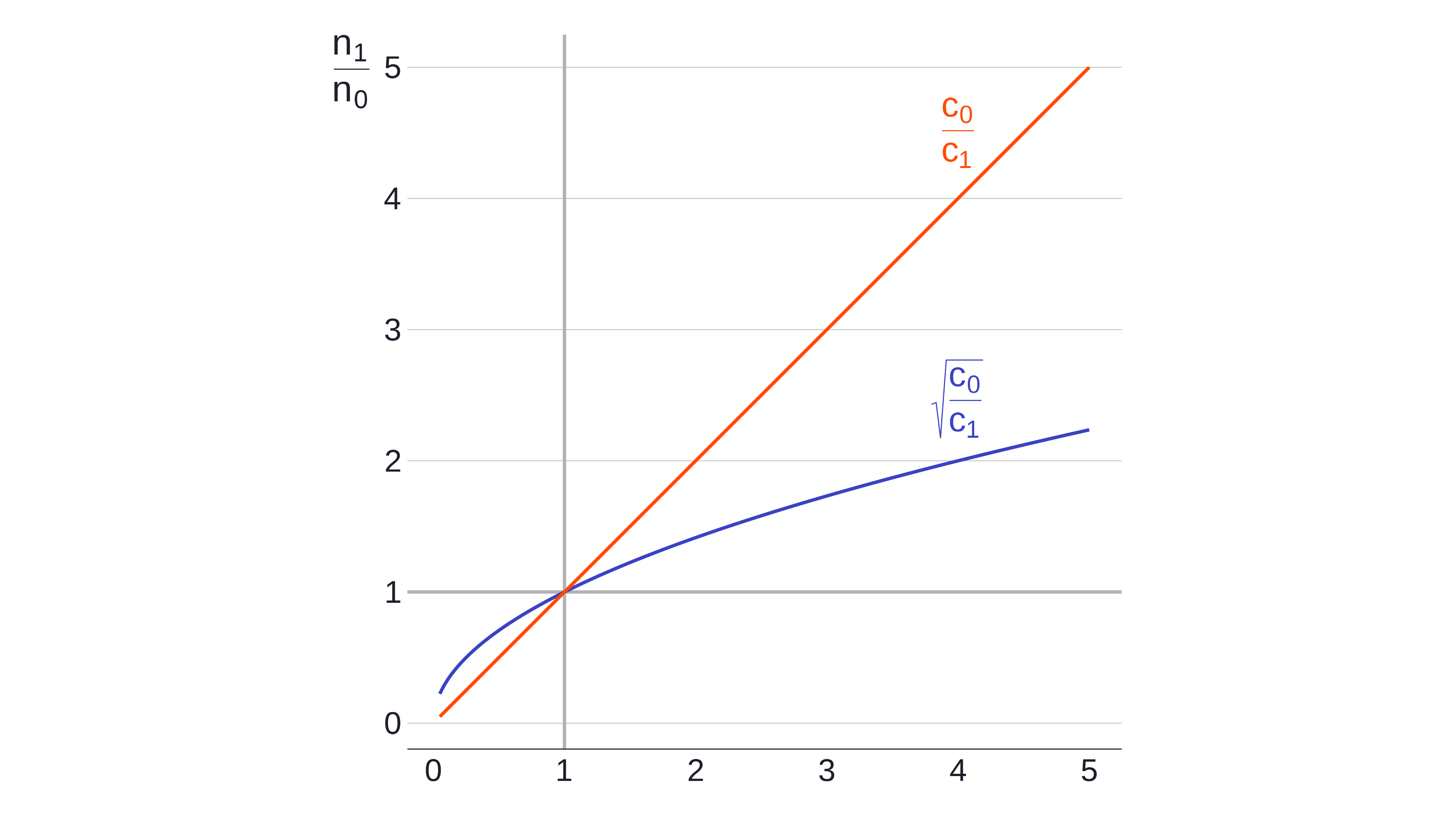
Intuition. Doubling the cost does not mean halving the allocation to the expensive arm. The twice-the-cost-half-the-subjects rule treats every subject as equally valuable, wherever they sit and however big the sample already is.
Question for you: is a subject’s contribution to precision actually constant? As sample size grows, precision gets higher, but incremental precision diminishes: every new subject will help less. That is what bends the rule away from a straight one-to-one with cost.
So, the answer is just that. It’s an easy heuristic, but it’s also a little cryptic stand-alone. So, of course you’d ask: why is that so, exactly? Why a square root, and not some other function with diminishing returns?
From wobbly averages to cost-optimal variant allocation
Your experiment estimates an effect by substracting the control group’s average outcome from the treatment group’s average outcome. Because you only sampled some subjects, each average has a given deviation (hence wobbly) with respect to the true average. Across many such sample averages, that wobble is measured by the variance of the mean, expressed as
where is the variance of the outcome at hand, and n is the sample size. Looks familiar yet? Take the square root of it, and you’d get the standard error of the mean.
Intuition. At a fixed sample size, n, we can be less certain about any estimate, e.g., the sample mean, the higher the variance of the outcomeis. But, turn it around and, with a fixed variance, the more samples we collect, the more certain we become about the estimate at hand. In other words, sample size offsets uncertainty in sample estimates coming from the variance in the outcome, .
Recall that we subtracting two averages. It happens to be that the variance of the treatment effect is the sum of the variances of the two arms at hand. Better-known yet as the variance of the difference-in-means estimator
where the two variances add plainly like this because the arms are independent samples under random assignment (a very ok assumption to make under an A/B test regime).is the sample average.is what we want to minimise, generally, so that we obtain high power.
Now comes a key point in the story. Sample allocation is about splitting the total pool of subjects into treatment and control groups. And the optimal allocation is one such that is as low as we can get it. That’s what optimal means here. The question is: how do we obtain such an optimal configuration; by allocating more to treatment or control?
The answer is: it depends, twice. First, it depends on the assumption of equal variances. Second, it depends on whether one is after the cost-optimal allocation. As the starting point of this all is hetergenous costs across arms, we can say that we are, indeed.
Let’s first clear up how the variance of each arm tells us something about the optimal allocation. With still in mind, we need to see what happens when an additional subject is allocated to one of the two groups. The below expression tells us that increasing the sample size results in a change in the variance of the estimator,
At high n, the increment of 1 is negligible (), so the expression simplifies to
this is our pay-off function in terms of per marginal n. We’re reasoning with one arm at a time, but recall that the is a function of two terms like the above one: one for control and one for treatment.
On with an example to make things concrete: say you are at 500 subjects, and the outcome has = 40, then adding 1 subject buys you a decrease of 40/500^2 = 0.00016 in . n comes in under a square in equation 5, so as n increases, a single unit increment pays off less, and less.
That’s an important point. Adding samples does not pay off in a consistent way: the more you have already, the less it helps to add one more sample. And there’s where the door opens to allocate that single sample differently; perhaps somewhere where it pays off more. But before we go there, let’s tailor this expression to our use case.
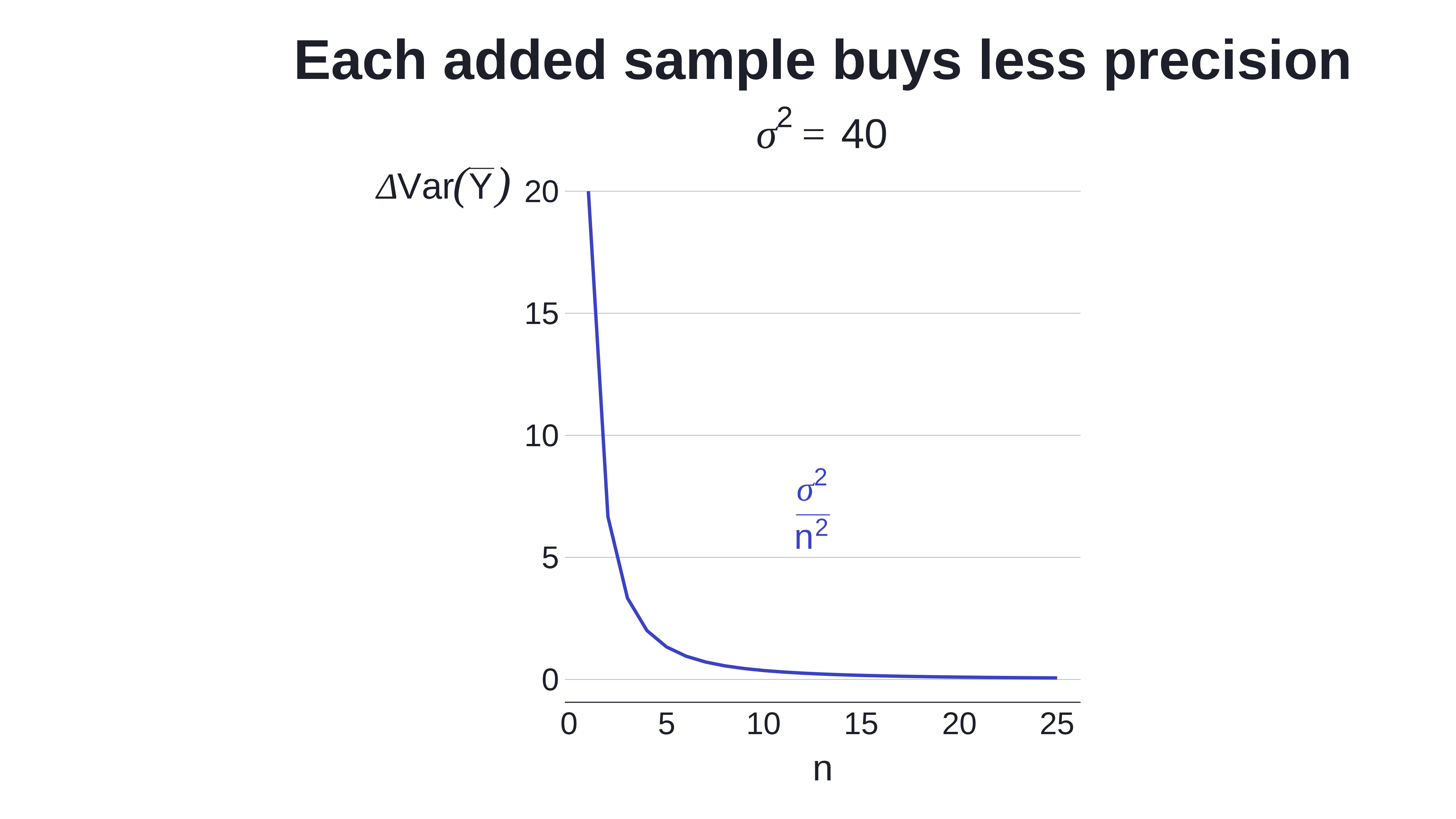
The current tells us the gains in precision per additional sample, but we are interested in gains in precision per dollar spent.
The bridge is simple: if a sample in a given arm costs c dollars, the precision you buy per dollar is the gain per sample divided by c. Bringing back the group index (1, 0) to make clear that cost may vary across arms, the expression for the treatment group becomes
Next is where we bring economic sense into allocating the next sample. We got the expression of precision-gains-per-dollar for each arm. We also know that an extra dollar stops bringing us much gain once we’ve reached a high sample size (or total spend) already; and moreover, the cost of that dollar may vary across the arms. In that case, the intuition says that we add a dollar to an arm when doing so brings more gains than allocating it to the other arm. In terms of optima, that’s the case when:
If we break this equality, it simply means that we are not indifferent to where we allocate the next dollar. We’d add it where the value is higher, and as we allocate an additional dollar there, allocating yet another dollar just became less interesting, by the diminishing returns we discussed above.
From here, the initial expression is two steps away. First we cross-multiply to get the n’s to the left:
Then, we take the square root to free the n’s from the power
There’s where we see how a square root came to be the diminishing returns mechanism. One can also see that under the assumption of equal variances across arms, we get the simpler and final:
Why assume such a thing? Because it’s reasonable to do so when traffic has been randomly allocated, and you have no a priori knowledge of the ratios in the experimental data. If we have reasons not to, then the ratio of standard deviations becomes co-author for the optimal sample ratio, indeed.
Full circle. And that’s it with the math for today.
Putting numbers on it
Say you work at an online travel agency, and the team wants to test an LLM-powered free-write search (“a beach town in Portugal, walkable, good coffee”) against the trusty filter-based one. Every user in the treatment arm fires off metered LLM calls as they search; over the course of the test, that adds up to about €0.20 per treated user, on average. The old search isn’t free either; its compute comes to roughly €0.05 per user. That’s a 4x cost ratio.
The rule says: . One treated user for every two controls; a 33/67 split, not 50/50, and not the 20/80 that “four times the price, a quarter of the users” would have suggested.
Say your power calculation at 50/50 asks for 20,000 users per arm:
-
50/50 (optimal runtime disregarding cost): 20,000 treated at €0.20, plus 20,000 controls at €0.05. Total: €5,000.
-
33/67 (cost-optimal runtime): the skew gives up a little sensitivity, so the total headcount grows to compensate; holding fixed with works out to 15,000 treated and 30,000 controls. Total: 15,000 at €0.20 plus 30,000 at €0.05 is €4,500.
That’s the same learning, with the same power, but the bill is 10% smaller. A tenth off may not sound like the heist of the century, but it’s a tenth of whatever the bill happens to be: millions in some cases. . We do pay in runtime, though: 12.5% more subjects overall. 12.5% more users could mean running an extra week; or 2 more days. Question: when would we be happy with saving a few thousands, or millions, and pay 1 extra week runtime in return?
Other complexities in real life
The heuristic is simple. Now we also know how it comes to be. But we need to zoom out to see how it works outside of the realm of math. Next I share three things I can think of that matter before going for the skewed split.
The power you “lose” comes back cheaper
One objection I’d raise myself is that skewing away from 50/50 loses power at a given runtime (and implied sample size), and without a hard constraint, e.g., runtime, total sample size, or budget, you’ll simply run longer to earn it back. Doesn’t the cost creep back in over that longer runtime?
It doesn’t because the extra runtime fills the cheap arm. We saw this in the section “putting numbers on it”: hold power fixed and watch the composition instead of the total. The skewed design needed 12.5% more subjects than 50/50, but treatment shrank by 25% while control grew by 50%.
What you do pay is calendar time; that’s the speed-versus-cost trade from the top of this post, in its most concrete form. But there is a very real and practical dimension to this tension that we need to consider: the relationship between runtime and sample size is not linear on most platforms. Daily users (say, 20% of your base) accrue fast over the first weeks, while we’d have to wait relatively longer for the less frequent users (the other 80%) to come in. Conversely, in the case of new users: these usually come in at a more or less fixed rate over time.
The issue is that the extra wait may become a much larger cost in terms of (learning) velocity than we can afford. Which makes this a tension between two types of costs: the monetary, directly measurable one vs. the indirect cost of longer learning cycles. This is an easy to overlook point that may make us feel good with ourselves (because look at us being optimal), but in the meantime hurt the business, or cause a conflict of interests between the speed devils and the accountants, among us.
The expensive arm is also your learning arm
Theidea shrinks the expensive arm, and that’s exactly where the trouble hides. Everything you want to learn about the treatment lives in the treatment group: the segment cuts, the guardrail metrics on treated users, the “who does this actually work for” questions. A split that is cost-optimal for the headline metric can leave you unable to answer any of the follow-ups.
So before committing, write down the secondary questions you’ll be asked in the readout, and check the smaller arm still powers the most granular one you care about. That gives you a floor on ; apply the cost rule above that floor.
You’ll save a bit less than the formula promised. In exchange, you won’t end the test with a significant top-line and a shrug for every question that follows.
Use the average marginal cost; and expect it to wobble
The formula wants the marginal cost of a treated subject, and with AI features that number is not a constant. Tokens vary per session, heavy users are disproportionally expensive, caching and retries move this marginal cost around. An average cost per user hides a fat tail, and the tail is where the money goes.
The move: estimate the marginal cost from a pilot or a small shadow rollout, and carry it as a range rather than a point. Then lean on a friendly property of the heuristic: the square root damps estimation error. A 4x versus 5x cost ratio is a big miss in accounting terms, but it barely moves the optimal split.
Get the cost ratio roughly right and move on; don’t stall the design chasing decimals the square root will flatten anyway.
Note: Fixed costs, like the build itself, a flat platform fee, a reserved-capacity contract, don’t change with allocation, so they can’t change the optimal one; only the per-user part of the bill belongs in .
Wrapping up
So, where does this leave us? The 50/50 split is not a law of nature; it’s the optimal answer to a design question that assumes both arms cost the same. The moment a treated subject costs more than a control one, that assumption breaks, and the optimal split moves: , leaning away from the expensive arm, with the square root keeping the lean gentle, even when the cost gap is not. Why start thinking about this now? With agentic features, and the cost of LLM-driven experiences, treating a user increasingly means paying for that user, session by session. The sample ratio is one of the few levers that acknowledges that at design time, before any bill exists.
Just as important is knowing when to leave the lever alone. If the cost ratio sits near 1, the square root flattens it into a split you couldn’t tell apart from 50/50; keep the default. If the treatment bill is small next to what the decision is worth, the optimisation won’t pay for the meeting where you explain the exotic ratio to your product manager. And when the team is starving for speed, remember what the skew charges: calendar time, and possibly the secondary deep-dive questions that live in the treated arm. In those cases, paying full price for the faster 50/50 answer is simply the better deal.
Always happy to pick up the conversation on LinkedIn. You can stay up to date with my writing by just visiting here often, or my personal blog.

Leave a Reply